Reducing Edge Artifacts in 2D Fourier Tranforms with Python
Aug, 2015
This tutorial is part of work published byHovden et al., Microsc. and Microanaly. (2015)
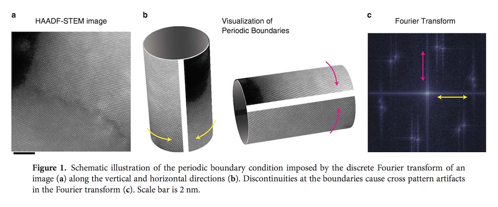
Abstract. The discrete Fourier transform is among the most routine tools used in high-resolution scanning/ transmission electron microscopy (S/TEM). However, when calculating a Fourier transform, periodic boundary conditions are imposed and sharp discontinuities between the edges of an image cause a cross patterned artifact along the reciprocal space axes. This artifact can interfere with the analysis of reciprocal lattice peaks of an atomic resolution image. Here we demonstrate that the recently developed Periodic Plus Smooth Decomposition technique provides a simple, efficient method for reliable removal of artifacts caused by edge discontinuities. In this method, edge artifacts are reduced by subtracting a smooth background that solves Poisson’s equation with boundary conditions set by the image’s edges. Unlike the traditional windowed Fourier transforms, Periodic Plus Smooth Decomposition maintains sharp reciprocal lattice peaks from the image’s entire field of view. [Manuscript]
Traditional Approach: Fourier Transform of Symmetrized Image In Python
One approach to obtaining continuity at the periodic boundaries is to symmetrize the image. Mirroring an image about the x, y directions ensures continuous boundary conditions and greatly reduces the cross pattern artifact in the DFT (Figs. 2b, 2g). However, this process adds symmetries that do not exist in the original image. Note that because the image size quadruples, there is a computational penalty—albeit manageable.
from pylab import *
#This function returns the Symmetrized Image FFT
def symfft2(im):
symim = zeros( [2*size(im,0), 2*size(im,1)] )
symim[0:size(im,0),0:size(im,1)] = im
symim[0:size(im,0),size(im,1):2*size(im,1)] = fliplr(im)
symim[size(im,0):2*size(im,0),0:size(im,1)] = flipud(im)
symim[size(im,0):2*size(im,0),size(im,1):2*size(im,1)] = flipud(fliplr(im))
return( fft2(symim) )
Traditional Approach: Windowed Fourier Transform in Python (2D)
A more common technique used in periodic artifact
reduction is a windowed Fourier transform. The window is
typically a smooth and continuous damping function with a
central maximum that decays to zero (or nearly zero) at the
edges of the image. This not only
removes the edge discontinuities—thus reducing the cross
pattern artifacts—but also reduces the background level (side
lobes) around each Fourier peak. A multitude of
window functions, each named to honor their inventor, have
been devised to achieve different advantages (Harris, 1978).
As the window function becomes more spatially confined in
real space, it degrades the resolution in reciprocal space.
A more deceptive consequence of using windowing for
artifact reduction is the unequal weighting it places on the
image. Regions toward the center of the image contribute
strongly to the Fourier spectrum and information toward the
edges of the field of view becomes negligible.
[Read More]
from pylab import *
#This function returns the Hann Windowed Fourier Transform
def hannfft(im):
window – outer( hanning(size(im,0)), hanning(size(im,1))
winim = window * im
return( fft2(winim) )
New Approach: Periodic Plus Smooth Decomposition in Python (2D)
One can substantially reduce the central cross pattern artifact caused by
periodic boundaries through implementation of the Periodic
Plus Smooth Decomposition (P + S) method. Altering only the low
frequencies, this approach provides an accurate estimation of
the Fourier spectrum in regions were atomic lattice Fourier
peaks occur—with contributions from the entire image field.
Moisan (2010) proposed a decomposition method
that removes the boundary artifacts while preserving
all the diffraction peaks from the entire image field of view.
Here, an image (u) is decomposed into a sum of a
“periodic” component (p) and a “smooth” component (s),
that is, u = p + s. Mathematically, the smooth component (s)
is obtained by solving Poisson's equation with
a boundary discontinuity image that captures the intensity
gaps across the edges of the original image. In general,
Poisson’s equation has a unique solution with slow spatial
variation. By subtracting s from the original image,
the periodic edge discontinuities are removed and the
information at higher frequencies is preserved.
[Read More]
from pylab import *
#This function returns the reciprocal space P and S components
def mfft2(im):
[rows,cols] = shape(im)
#Compute boundary conditions
s = zeros( shape(im) )
s[0,0:] = im[0,0:] - im[rows-1,0:]
s[rows-1,0:] = -s[0,0:]
s[0:,0] = s[0:,0] + im[0:,0] - im[:,cols-1]
s[0:,cols-1] = s[0:,cols-1] - im[0:,0] + im[:,cols-1]
#Create grid for computing Poisson solution
[cx, cy] = meshgrid(2*pi*arange(0,cols)/cols, 2*pi*arange(0,rows)/rows)
#Generate smooth component from Poisson Eq with boundary condition
D = (2*(2 - cos(cx) - cos(cy)))
D[0,0] = inf # Enforce 0 mean & handle div by zero
S = fft2(s)/D
P = fft2(im) - S # FFT of periodic component
return(P,S)